![]()
Plot INCA data
In this jupyter notebook, we will show how to import and plot a precipitation forecast from the INCA nowcasting system.
Install dependencies
First, let’s set up our working environment. It is recommended to use a virtual environment.
Important: In Google Colab, this notebook needs to be executed one cell at a time. Trying to excecute all the cells at once may results in cells being skipped and some dependencies not being installed.
Now, let’s install the dependendies that will allow us to read and visualize the example data. To do so, we will use two main python packages: xarray to work with labelled multi-dimensional arrays, and matplotlib for visualization.
[1]:
!pip install xarray matplotlib
Collecting xarray
  Downloading xarray-0.20.2-py3-none-any.whl (845 kB)
     |████████████████████████████████| 845 kB 4.5 MB/s
Requirement already satisfied: matplotlib in /home/docs/checkouts/readthedocs.org/user_builds/inca-examples/conda/latest/lib/python3.9/site-packages (3.5.1)
Requirement already satisfied: numpy>=1.18 in /home/docs/checkouts/readthedocs.org/user_builds/inca-examples/conda/latest/lib/python3.9/site-packages (from xarray) (1.20.3)
Collecting pandas>=1.1
  Downloading pandas-1.3.5-cp39-cp39-manylinux_2_17_x86_64.manylinux2014_x86_64.whl (11.5 MB)
     |████████████████████████████████| 11.5 MB 49.9 MB/s
Requirement already satisfied: python-dateutil>=2.7 in /home/docs/checkouts/readthedocs.org/user_builds/inca-examples/conda/latest/lib/python3.9/site-packages (from matplotlib) (2.8.2)
Requirement already satisfied: fonttools>=4.22.0 in /home/docs/checkouts/readthedocs.org/user_builds/inca-examples/conda/latest/lib/python3.9/site-packages (from matplotlib) (4.28.3)
Requirement already satisfied: packaging>=20.0 in /home/docs/checkouts/readthedocs.org/user_builds/inca-examples/conda/latest/lib/python3.9/site-packages (from matplotlib) (21.3)
Requirement already satisfied: pillow>=6.2.0 in /home/docs/checkouts/readthedocs.org/user_builds/inca-examples/conda/latest/lib/python3.9/site-packages (from matplotlib) (8.4.0)
Requirement already satisfied: kiwisolver>=1.0.1 in /home/docs/checkouts/readthedocs.org/user_builds/inca-examples/conda/latest/lib/python3.9/site-packages (from matplotlib) (1.3.2)
Requirement already satisfied: cycler>=0.10 in /home/docs/checkouts/readthedocs.org/user_builds/inca-examples/conda/latest/lib/python3.9/site-packages (from matplotlib) (0.11.0)
Requirement already satisfied: pyparsing>=2.2.1 in /home/docs/checkouts/readthedocs.org/user_builds/inca-examples/conda/latest/lib/python3.9/site-packages (from matplotlib) (3.0.6)
Requirement already satisfied: pytz>=2017.3 in /home/docs/checkouts/readthedocs.org/user_builds/inca-examples/conda/latest/lib/python3.9/site-packages (from pandas>=1.1->xarray) (2021.3)
Requirement already satisfied: six>=1.5 in /home/docs/checkouts/readthedocs.org/user_builds/inca-examples/conda/latest/lib/python3.9/site-packages (from python-dateutil>=2.7->matplotlib) (1.16.0)
Installing collected packages: pandas, xarray
Successfully installed pandas-1.3.5 xarray-0.20.2
Download the data
Now that we have the environment ready, let’s download an example dataset.
On Zenodo, we can download the ouput from a single run of INCA for precipitation (mm/h).
[2]:
!wget https://zenodo.org/record/5575197/files/RR_INCA.nc
--2021-12-15 18:01:17--  https://zenodo.org/record/5575197/files/RR_INCA.nc
Resolving zenodo.org (zenodo.org)... 137.138.76.77
Connecting to zenodo.org (zenodo.org)|137.138.76.77|:443... connected.
HTTP request sent, awaiting response... 200 OK
Length: 5887704 (5.6M) [application/octet-stream]
Saving to: ‘RR_INCA.nc’

RR_INCA.nc          100%[===================>]   5.61M  6.16MB/s    in 0.9s

2021-12-15 18:01:19 (6.16 MB/s) - ‘RR_INCA.nc’ saved [5887704/5887704]
Read the data
Now that we have downloaded the example data, let’s import the example netCDF with xarray.open_dataset() method.
The file is called RR_INCA.nc. “RR” is the product name used to identify the quantitative precipitation nowcasting product based on the merging between radar and station observations (named CombiPrecip). This product is in units of mm/h, it is updated every 10 minutes, and it has a 6 hour forecast range.
We import this 6-hour precipitation forecast, which corresponds to a sequence of 37 frames of 10-min precipitation fields (1 analysis and 36 forecasts).
[3]:
import xarray as xr

ds = xr.open_dataset("RR_INCA.nc")
ds
Matplotlib is building the font cache; this may take a moment.
[3]:
<xarray.Dataset>
Dimensions:       (chx: 710, chy: 640, time: 37)
Coordinates:
  * chx           (chx) float64 2.555e+05 2.565e+05 ... 9.635e+05 9.645e+05
  * chy           (chy) float64 -1.595e+05 -1.585e+05 ... 4.785e+05 4.795e+05
  * time          (time) datetime64[ns] 2021-07-08T08:20:00 ... 2021-07-08T14...
Data variables:
    RR            (time, chy, chx) float32 ...
    grid_mapping  float32 9.969e+36
Attributes:
    conventions:     CF-1.6
    conventionsURL:  http://cfconventions.org/cf-conventions/v1.6.0/cf-conven...
    title:           simple NetCDF output
    institution:     MeteoSwiss (NMC Switzerland)
    source:          model: inca-1,product_category: determinist, version: 3.2
    reference:       MeteoSwiss (2021)
    history:         Produced by inca2netcdf 1.0 on 2021-07-08 08:30 UTC
comment: Illustrate simplified NetCDF structure when all fields d...Basic plotting
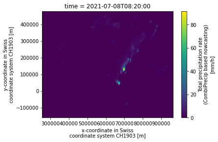
Xarray’s includes some plotting functionalities that we can use to visualize our example data.
[4]:
precip_field = ds.RR.isel(time=0) # select the first rainfall field, that is, the analysis
precip_field.plot()
[4]:
<matplotlib.collections.QuadMesh at 0x7f54d8a2d520>
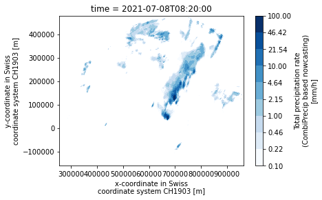
One can easily add transparency to the dry areas and customize the colormap.
[5]:
import numpy as np

levels = np.logspace(-1, 2, 10, base=10)
cmap = "Blues"
precip_field.where(precip_field >= 0.1).plot(levels=levels, cmap=cmap)
[5]:
<matplotlib.collections.QuadMesh at 0x7f54d88e0820>
Plot with Cartopy
Cartopy is a python library for plotting georeferenced datasets and maps.
Installing Cartopy is a bit more involved as it requires few additonal library dependencies. Also, shapely need to be reinstalled by ignoring the binary wheels to make it compatible with Cartopy.
[6]:
!apt-get install -qq libgdal-dev libgeos-dev
!pip uninstall --yes shapely
!pip install shapely --no-binary shapely
!pip install cartopy pyepsg
E: Could not open lock file /var/lib/dpkg/lock-frontend - open (13: Permission denied)
E: Unable to acquire the dpkg frontend lock (/var/lib/dpkg/lock-frontend), are you root?
Found existing installation: Shapely 1.8.0
Uninstalling Shapely-1.8.0:
  Successfully uninstalled Shapely-1.8.0
Collecting shapely
  Downloading Shapely-1.8.0.tar.gz (278 kB)
     |████████████████████████████████| 278 kB 4.6 MB/s
  Preparing metadata (setup.py) ... - done
Skipping wheel build for shapely, due to binaries being disabled for it.
Installing collected packages: shapely
    Running setup.py install for shapely ... - \ | / done
Successfully installed shapely-1.8.0
Requirement already satisfied: cartopy in /home/docs/checkouts/readthedocs.org/user_builds/inca-examples/conda/latest/lib/python3.9/site-packages (0.20.1)
Collecting pyepsg
  Downloading pyepsg-0.4.0-py3-none-any.whl (6.0 kB)
Requirement already satisfied: pyshp>=2.1 in /home/docs/checkouts/readthedocs.org/user_builds/inca-examples/conda/latest/lib/python3.9/site-packages (from cartopy) (2.1.3)
Requirement already satisfied: numpy>=1.18 in /home/docs/checkouts/readthedocs.org/user_builds/inca-examples/conda/latest/lib/python3.9/site-packages (from cartopy) (1.20.3)
Requirement already satisfied: pyproj>=3.0.0 in /home/docs/checkouts/readthedocs.org/user_builds/inca-examples/conda/latest/lib/python3.9/site-packages (from cartopy) (3.3.0)
Requirement already satisfied: shapely>=1.6.4 in /home/docs/checkouts/readthedocs.org/user_builds/inca-examples/conda/latest/lib/python3.9/site-packages (from cartopy) (1.8.0)
Requirement already satisfied: matplotlib>=3.1 in /home/docs/checkouts/readthedocs.org/user_builds/inca-examples/conda/latest/lib/python3.9/site-packages (from cartopy) (3.5.1)
Requirement already satisfied: requests in /home/docs/checkouts/readthedocs.org/user_builds/inca-examples/conda/latest/lib/python3.9/site-packages (from pyepsg) (2.26.0)
Requirement already satisfied: fonttools>=4.22.0 in /home/docs/checkouts/readthedocs.org/user_builds/inca-examples/conda/latest/lib/python3.9/site-packages (from matplotlib>=3.1->cartopy) (4.28.3)
Requirement already satisfied: kiwisolver>=1.0.1 in /home/docs/checkouts/readthedocs.org/user_builds/inca-examples/conda/latest/lib/python3.9/site-packages (from matplotlib>=3.1->cartopy) (1.3.2)
Requirement already satisfied: python-dateutil>=2.7 in /home/docs/checkouts/readthedocs.org/user_builds/inca-examples/conda/latest/lib/python3.9/site-packages (from matplotlib>=3.1->cartopy) (2.8.2)
Requirement already satisfied: packaging>=20.0 in /home/docs/checkouts/readthedocs.org/user_builds/inca-examples/conda/latest/lib/python3.9/site-packages (from matplotlib>=3.1->cartopy) (21.3)
Requirement already satisfied: cycler>=0.10 in /home/docs/checkouts/readthedocs.org/user_builds/inca-examples/conda/latest/lib/python3.9/site-packages (from matplotlib>=3.1->cartopy) (0.11.0)
Requirement already satisfied: pillow>=6.2.0 in /home/docs/checkouts/readthedocs.org/user_builds/inca-examples/conda/latest/lib/python3.9/site-packages (from matplotlib>=3.1->cartopy) (8.4.0)
Requirement already satisfied: pyparsing>=2.2.1 in /home/docs/checkouts/readthedocs.org/user_builds/inca-examples/conda/latest/lib/python3.9/site-packages (from matplotlib>=3.1->cartopy) (3.0.6)
Requirement already satisfied: certifi in /home/docs/checkouts/readthedocs.org/user_builds/inca-examples/conda/latest/lib/python3.9/site-packages (from pyproj>=3.0.0->cartopy) (2021.10.8)
Requirement already satisfied: urllib3<1.27,>=1.21.1 in /home/docs/checkouts/readthedocs.org/user_builds/inca-examples/conda/latest/lib/python3.9/site-packages (from requests->pyepsg) (1.26.7)
Requirement already satisfied: charset-normalizer~=2.0.0 in /home/docs/checkouts/readthedocs.org/user_builds/inca-examples/conda/latest/lib/python3.9/site-packages (from requests->pyepsg) (2.0.9)
Requirement already satisfied: idna<4,>=2.5 in /home/docs/checkouts/readthedocs.org/user_builds/inca-examples/conda/latest/lib/python3.9/site-packages (from requests->pyepsg) (3.1)
Requirement already satisfied: six>=1.5 in /home/docs/checkouts/readthedocs.org/user_builds/inca-examples/conda/latest/lib/python3.9/site-packages (from python-dateutil>=2.7->matplotlib>=3.1->cartopy) (1.16.0)
Installing collected packages: pyepsg
Successfully installed pyepsg-0.4.0
We first define a method to plot reference geographical features to an existing figure axis.
[7]:
import cartopy.crs as ccrs
import cartopy.feature as cfeature

def add_geo_features(ax):
    """
    Add reference geographical layers such as thenational boundaries
    and the main lakes and rivers.
    """
    ax.add_feature(
        cfeature.NaturalEarthFeature(
            "cultural",
            "admin_0_boundary_lines_land",
            scale="10m",
            edgecolor="black",
            facecolor="none",
            linewidth=1,
        )
    )
    ax.add_feature(
        cfeature.NaturalEarthFeature(
            "physical",
            "rivers_lake_centerlines",
            scale="10m",
            edgecolor=np.array([0.59375, 0.71484375, 0.8828125]),
            facecolor="none",
            linewidth=1,
        )
    )
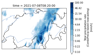
To use Cartopy, we need to specify the source and target coordinate reference system. In our case, the Swiss coordinate system CH1903/LV03 can be identified by the EPSG 21781.
[8]:
crs = ccrs.epsg(21781)

# plot the precipitation field on the original Swiss projection
ax = precip_field.where(precip_field > 0).plot(
    transform=crs,
    subplot_kws=dict(projection=crs),
    levels=levels,
    cmap=cmap
    ).axes
add_geo_features(ax)
/home/docs/checkouts/readthedocs.org/user_builds/inca-examples/conda/latest/lib/python3.9/site-packages/cartopy/crs.py:825: ShapelyDeprecationWarning: __len__ for multi-part geometries is deprecated and will be removed in Shapely 2.0. Check the length of the `geoms` property instead to get the  number of parts of a multi-part geometry.
  if len(multi_line_string) > 1:
/home/docs/checkouts/readthedocs.org/user_builds/inca-examples/conda/latest/lib/python3.9/site-packages/cartopy/crs.py:877: ShapelyDeprecationWarning: Iteration over multi-part geometries is deprecated and will be removed in Shapely 2.0. Use the `geoms` property to access the constituent parts of a multi-part geometry.
  for line in multi_line_string:
/home/docs/checkouts/readthedocs.org/user_builds/inca-examples/conda/latest/lib/python3.9/site-packages/cartopy/crs.py:944: ShapelyDeprecationWarning: __len__ for multi-part geometries is deprecated and will be removed in Shapely 2.0. Check the length of the `geoms` property instead to get the  number of parts of a multi-part geometry.
  if len(p_mline) > 0:
/home/docs/checkouts/readthedocs.org/user_builds/inca-examples/conda/latest/lib/python3.9/site-packages/cartopy/io/__init__.py:241: DownloadWarning: Downloading: https://naturalearth.s3.amazonaws.com/10m_cultural/ne_10m_admin_0_boundary_lines_land.zip
  warnings.warn(f'Downloading: {url}', DownloadWarning)
/home/docs/checkouts/readthedocs.org/user_builds/inca-examples/conda/latest/lib/python3.9/site-packages/cartopy/io/__init__.py:241: DownloadWarning: Downloading: https://naturalearth.s3.amazonaws.com/10m_physical/ne_10m_rivers_lake_centerlines.zip
  warnings.warn(f'Downloading: {url}', DownloadWarning)
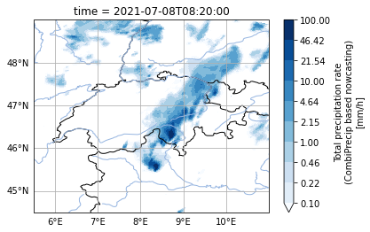
With Cartopy, we can easily switch to alternative geographical projections, here for example using Plate Carrée.
[9]:
# plot the precipitation field on the Plate Carrée projection
ax = precip_field.where(precip_field > 0).plot(
    transform=crs,
    subplot_kws=dict(projection=ccrs.PlateCarree()),
    levels=levels,
    cmap=cmap
    ).axes
add_geo_features(ax)

# draw lat lon lines
grid_lines = ax.gridlines(
    crs=ccrs.PlateCarree(),
    draw_labels=True,
    dms=True
)
grid_lines.top_labels = grid_lines.right_labels = False
grid_lines.y_inline = grid_lines.x_inline = False
grid_lines.rotate_labels = False

# zoom on the map
ax.set_extent([5.5, 11, 44.5, 49])